3.1 Query specification for multiple regression analysis
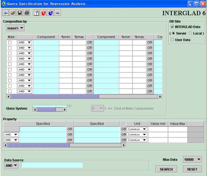
The prediction of properties is conducted by multiple regression analysis. Click on [Go Prediction] in the main window, and then click on [Regression Analysis] button in the prediction menu. The [Query Specification for Regression Analysis] window appears. Query specifications are inputted to collect the existing data to serve as the basis for a prediction. The Glass State for such predictions is only 'Glass'.
(1) Replacement of database
Select the INTERGLAD or user database. Both databases can be used together, if desired. As for the INTERGLAD database, select either the latest version on the server or the version on the user's personal computer. The selection can be changed using the [User Environment] menu opened by clicking on the [User Environment] icon in the main window.
In the Applet version, only data on the server can be used.
(2) Query specification
1) Component
| a) | Unit pull-down menu The unit for the composition can be selected from among mass%, mol% or at%. The default unit is mass%, but this can be changed using the [User Environment] menu. |
| b) | Component Any component can be chosen from the dialog box opened by clicking in any light blue cell of the Component column. Non-numerical compositional data are not retrieved. Glasses without the component can be extracted by inputting "-1" in the [%min] cell. This is convenient when even small amounts of an unwanted component are retrieved. |
| c) | Total of main component [  Total of Main Component] becomes effective only when the adjacent [Main]
checkbox is checked and the total content of the main component can be
specified. When this option is specified, the vertical OR and NOT operators
and the horizontal OR operator cannot be used.d) Glass system Total of Main Component] becomes effective only when the adjacent [Main]
checkbox is checked and the total content of the main component can be
specified. When this option is specified, the vertical OR and NOT operators
and the horizontal OR operator cannot be used.d) Glass systemThe glass system can be selected from the list opened by double-clicking in a light blue [Glass System] cell. |
2) Property
The property specified here is used for the multiple regression analysis. Up to three properties can be specified for simultaneous use.
Properties can be selected from the dialog box opened by double-clicking in a light blue cell of the [Property] column.
The unit system - Common, SI, CGS or PSI - can be separately specified for each property. (The default unit is Common, but this default can be changed using the User Environment preferences accessed through the main window.
By choosing an item higher on the [Property] dialog list, a group of properties subordinate to the chosen property is used together for retrieval. When plural properties are found, one item among them is displayed.
Either AND or OR can be specified for each lines of the [Property] column.
[About retrieval for multiple regression analysis according to properties]
There are three retrieval modes as follows:
Each differs from the others in the process of multiple regression analysis.
| a) | Specifying with horizontal OR operator Left-hand cells take precedence over right-hand cells when plural properties are specified in a line. Property items that can be specified horizontally by the OR operator are limited to those of the same classification. The data are shown in the same column of the [Glasses for Regression Analysis] table. |
| b) | Specifying with vertical AND operator When the retrieval conditions are specified vertically with the AND operator, as all the retrieved glasses must have values for the same property item, the population of each property item for the regression analysis will be composed of a group of data. Therefore, the relation among several predicted property values can be expected to have high reliability. However, as the data to be collected is more tightly limited, the number of cases in which multiple regression analysis is impossible increase. |
| c) | Specifying with vertical OR operator When the retrieval conditions are specified vertically with the OR operator, not all retrieved glasses need have every property value specified for the prediction. It is possible that the population for the multiple regression analysis will be composed of groups differing from each other in property data. Therefore, the relationship among the predicted values for each property becomes more tenuous. Specifying retrieval conditions with the vertical OR operator is thus recommended only for compositions and properties for which data is limited. |
[About electric conductivity, AC resistivity and DC resistivity]
When electric conductivity, AC resistivity or DC resistivity is specified as a retrieval condition for regression analysis, other properties not specified also become conditions, according to the following table. When plural properties are retrieved, single data is listed in the [Glasses for Regression Analysis] window according to the priority levels in the following table.
|
Specified item
|
Priority 1
|
Priority 2
|
Priority 3
|
|
Electric conductivity
|
Electric conductivity
|
Reciprocal of AC resistivity
|
Reciprocal of DC resistivity
|
|
AC volume resistivity
|
AC volume resistivity
|
Reciprocal of conductivity
|
DC volume resistivity
|
|
DC volume resistivity
|
DC volume resistivity
|
Reciprocal of conductivity
|
AC volume resistivity
|
(3) Data Source
Data source category (data book / journal / proceedings / patent / catalogue) or items subordinate to these categories can be selected to specify sources. It is possible to exclude a certain data source by using the NOT operator.
(4) Max data
This is the upper limit to the number of retrieved glasses. The default limit is ten. However, this limit can be changed using the User Environment preferences accessed through the main window.
(5) [Search] button
Click to start the search.
(6) [Reset] button
Clear all inputted specifications.
[Explanation of functions]
(1) Search
Click the [Search] button to initiate the retrieval under the conditions specified in the query window. The database to be searched can be changed via the [DB site] column to the top-right of the window. The default database is the INTERGLAD database on the server. This default can be changed using the User Environment preferences accessed through the main window.
(2)
 [Save] icon
 The retrieval conditions on the window are saved in a file with the extension '.igd'. 'Query' is automatically given as the file name, but this name can be changed to any name of the user’s choice.
(3)
 [Open] icon
 A saved retrieval conditions file of type '.igd' is opened on the window.
(4)
 [Print] icon
 The window is printed as it appears.
The retrieval is conducted based on the retrieval conditions specified in the query specification window, and all retrieved glasses are shown in the order of their respective glass numbers. The multiple regression analysis is conducted using those data.
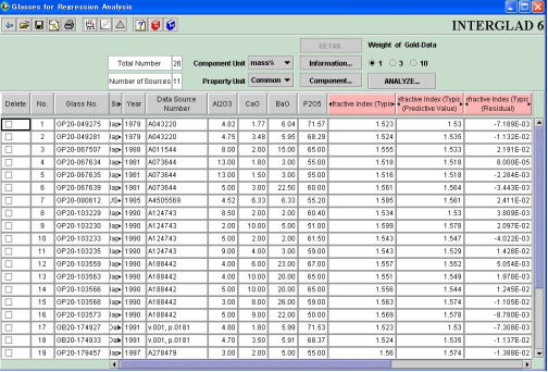
(1) General
1) Total Number: The total number of retrieved glasses
2) Number of sources: The total number of data sources for the retrieved glasses
(2) Table
Each datum is shown in a line according to its respective glass number. Only data concerning the specified items are tabulated, except for glass numbers and data sources. The table provides for the following operational functions:
| * | Replacement of columns: Any composition or property column can be moved to another position by dragging & dropping its label. |
| * | Sort order: The data in a column can be sorted according to ascending or descending order by 'shift-clicking' the column label. (This changes the order of the line from their original glass-number order.) |
| * | Transition to detailed window: It is possible to change to a detailed window by double-clicking the line. |
Glass data with the [Delete] checkbox checked are not used for the regression analysis. (A checkbox is checked automatically if its plot-point is deleted in the validity test window. See below.).
2) Number column
3) Glass number
4) Data source
The name of the data source, year and data source number appears in this column. They may be canceled by clicking the checkboxes for those items in the list box obtained by pressing the [Information …] button at the upper right of the window.
5) Composition
When any glass contains a component specified in the query specification window, that component is shown in a column. Other components not specified in the query specification window may be viewed by checking the appropriate checkbox of the list box opened by clicking the [Component …] button.
6) Property
The property specified in the query specification window is shown. New property items cannot be added on this window. Each property is shown in three columns, which give the measured and predictive values, as well as the residual. The color of the label is different in each property.
| * | Measured value This is the data extracted from the database. Blue-colored values are conditional data; it is recommended that the conditions for these data be confirmed in the detail window. Red-colored property values are data of priority levels 2 and 3 for electrical conductivity, AC resistivity and DC resistivity |
| * | Predictive Value This is the value derived by use of the equation obtained by the multiple regression analysis. The predictive value is calculated for the glass independently of the measured value. |
| * | Residual This is the difference between the measured and predictive values. |
The unit system for the property in question is 'Common' by default, and is not the unit system specified in the query specification window. The default can be set to another unit system by changing the [User Environment] preferences accessed through the main window.
(1) [Component Unit] pull-down menu
Conversion between mol% and mass% compositions is possible using the [Component Unit] pull-down menu. Conversion is impossible in cases where a glass contains a component for which the molecular weight is uncertain, such as R2O and kaolin, so the numerical data existing before conversion are replaced by a red asterisk '*'. The regression analysis does not use non-numerical data ( '*').
(2) [Property Unit] pull-down menu
Click to change the property unit and convert the property value.
(3) [DETAIL] button
Click to show the detail window for a selected glass. Select any line by clicking anywhere in it other than the deletion checkbox.
(4) [Information…] button
Click to show or hide the following items: Glass State, Glass System, Data Source information, Usage, Shape, etc.
(5) [Component…] button
Click to show or hide any component contained in the glass. The components (explanatory variables) used for the multiple regression analysis are only those shown in the retrieved glasses table.
(6) [Analyze…] button
The predictive values and residuals are derived by conducting the multiple regression analysis.
Click the [Analyze…] button to call up a dialog box, and press [OK] button in the box to start the multiple regression analysis.
The multiple regression analysis cannot be conducted when the number of sample glass is less than that of the explanatory variables (components) plus 2. A message warning that the accuracy may be low is shown when the number of sample glass is equal to the number of explanatory variables plus 3. A warning is also given when the number of glass for each explanatory variable is not more than 2.
Click the [Component …] button to show or hide any component.
When the show/hide condition of a component or the unit system is changed after [Analyze…] operation, the predictive values and residuals becomes invalid, so it is necessary to do the [Analyze…] operation over again.
The multiple regression analysis includes the equation (k = 0) when not using a constant, and the equation (k ≠ 0) when using one. Click the [Analyze…] button to call up a dialog box, select either equation in the box, and press the [OK] button.
The equation is usually used with a constant (k ≠ 0). A multiple regression analysis using a constant is conducted only for glass components displayed in the retrieval results list. The prediction property value is given by the following equation:
y = Σaixi+ k
On the other hand, the equation k = 0 can also be chosen. In this case, the multiple regression analysis includes components which are not displayed in the list, although the glass data are limited to those in which the total of those components does not exceed 10%. Such components are treated as a single component. The prediction property value is given by the following equation.
y = Σai xi + axxx
where, 'ax' is a coefficient of those components, and 'xx' is the amount of the total.
Attention: If a multiple regression analysis concerning all components (n) when the glass data consists of a maximum of n components are desired, the equation of k = 0 is recommended.
(7) [Weight of Gold-Data]
The multiple regression analysis is conducted with extra weight given to Gold-Data. Relative weightings may be selected from among 1, 3 and 10. The default weight is 1 (no extra weight).
(8)
[Save] iconClick on the [Save] icon to save the window. The file is automatically named "list", but this can be changed to any name desired by the user. The extension '.ige' is automatically appended.
(9)
[Open] icon Click on the [Open] icon to open the list of files with extension '.ige', then click the desired file name. Click the
(10)
[Print] iconClick on the [Print] icon to print the window.
[Window Navigation]
(1)
 [Composition Optimization] icon
After conducting the multiple regression analysis, choose any glass in the table and click on the [Composition Optimization] icon. Input a target value in the dialog box that appears. The [Property Prediction: Composition Optimization] window is opened.
An alert is shown when the [Composition Optimization] icon is clicked without previously selecting a glass.
(2)
 [Validity Test] icon
Choose any property in the dialog box shown by pressing the [Validity Test] icon. The [Property Prediction Validity Test] window opens.
(3)
Clicking on the [Ternary Plot] icon opens a dialog box. After selecting the three components and a property, the Ternary plot window appears.
(4)
Click on the [CSV File] icon to save the result of the retrieval as a CSV file. A dialog box showing the saving options appears when the [Save] icon is clicked.
<Saving options>
| * | Selection of columns to be saved: Choose those data items to be saved from the list that appears after clicking on the Component, Property or Information tag. |
| * | File name: Saved files are automatically named 'Glass', but this name can be changed. The file-type extension '.csv' is appended automatically. |
The property values of an arbitrary composition are calculated using the property prediction equation obtained from a multiple regression analysis, with the optimal composition being predicted by analysis of the multiple regression coefficients and the differences between the calculated and target values.
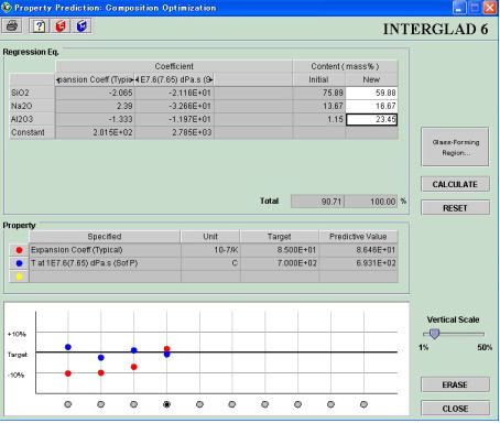
(1) Regression equation table
The lines and columns of this table are as follows:
Lines : component names and constant.
The components are those specified for multiple regression analysis.
Columns: the property names (up to three), the initial composition and the calculated (New) composition.
The coefficients of multiple regression equations for each component are shown in the columns. The composition of the glass selected on the former window is shown as the initial composition. When no glass is selected, this column is empty. New glass compositions may be freely inputted. The total of the glass components is not necessarily 100%.
(2) Property table
The lines and columns of this table are as follows:
Lines : property names (maximum three lines)
Columns: Target values and predictive values
The values specified in the dialog box are shown in the [Target] column. The values in the [Predictive value] column are obtained by pressing the [Calculate] button.
(3) Graphic display of property prediction
The quotient of the difference between the predictive and target values of a property divided by the target value is shown on this graph. The horizontal line in the middle of the table represents the target value. The vertical scale can be changed by from 1 to 50% using the slider to the right of the graph. The radio buttons at the bottom of the graph allow for multiple trials, with the number of plots increasing with each trial.
The initial plot corresponds to the property values of the initially specified glass in the previous window.
Different colors are assigned to the plot-points as shown at the left of the [Property] table.
(1) [Calculate] button
Click the [Calculate] button after inputting numerical values in the content column. The glass composition is first proportionally converted to values totaling 100% and then its properties are calculated. The results are shown in the [Property] table and the property prediction graph.
The number of trials shown on the graph is initially ten, but the plots shifts to the left to allow for more than ten trials. When the number of trials exceeds ten, the left-most plot is deleted and the latest plot appears at the right.
(2) [Glass-forming Region] button
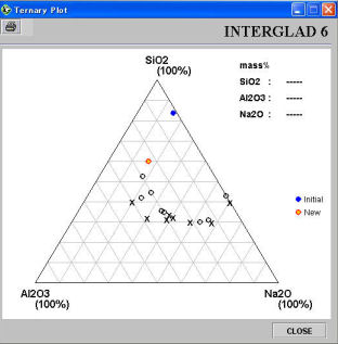
Clicking on this button calls up a dialog box. When three components are specified in the box, a ternary diagram showing the glass-forming region appears. This is used to confirm whether or not the optimal glass composition actually forms a glass or not.
Because three components totaling less than 100% are converted proportionally to total 100%, the further the initial sum departs from 100%, the less the reliability. The initial plot in the ternary diagram corresponds to the composition of the glass initially specified glass in the [Prediction: Retrieved Glasses] window.
The glass-forming range is shown with factual data. A completely transparent glass is denoted by a circle "o", while the glass composition falling just short of yielding transparent glass is denoted by an "x". The region to the circle-side of the mid-line between the circle "o" and the "x" is the glass-forming region.
Glass-forming region data are shown only at the boundaries, and not for individual data.
(3) Radio button in the property prediction graph
Click any radio button. The glass composition and property represented by the button are displayed in the Regression equation table and the [Property] table, respectively.
(4) [Erase] button
Click the [Erase] button to erase any plot for which the radio button is turned on; the plots to the deleted plot’s right move leftward to fill the vacancy. However, the initial plot cannot be deleted.
(5)
[Print] iconClick on the [Print] icon to print the window as it appears.
Comparison between the property values of the retrieved glasses specified in the query specification window and those resulting from multiple regression analyses based on the retrieved glasses is represented as a graph in order to verify the property prediction.
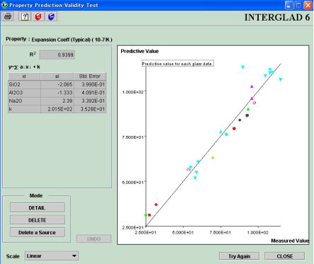
(1) Graph
The data is plotted on an X-Y chart on which the X and Y axes indicate the factual data and the predictive values resulting from multiple regression analysis, respectively. Each datum is given a different mark and color according to its data source. A yellow star indicates Gold-Data. Pointing the cursor at a plot-point displays its data number, glass number and data source in a balloon.
(2) Contribution rate (R2), coefficients of multiple regression analysis, and standard error
The contribution rate, the coefficients of multiple regression analysis, and the standard error are shown.
The predictive equation of the multiple regression analysis is
y = Σaixi + k or y = Σaixi + axxx
where y is the property value, ai the i'th coefficient of the multiple regression analysis, xi the content of i'th component, and k the constant, and ax the other-component's coefficient of the multiple regression analysis.
[Concerning the evaluation of a multiple regression analysis]
Although there are many kinds of criteria for the evaluation of multiple regression analysis, this system adopts the following four:
1) Graph
The predictive values can be compared with the measured values by means of the X-Y graph. If the predictive values coincide with the measured values, all plot-points fall on a line inclined 45 degrees to both axes. The accuracy of the prediction can be gauged roughly by viewing the dispersion of the plots around the 45-degree mid-line.
2) Regression coefficients (ai)
The magnitude of each coefficient of a multiple regression analysis indicates the order of influence of a given component.
3) Contribution rate (R2)
The contribution rate can be obtained by using the sum of the square of the difference between the measured and predictive values, and the sum of the square of each deviation (the difference between measured and mean values of the measured value). The greater the accuracy of the analysis, the smaller the residuals. When the ratio of the sum of the square of every residual to the sum of the square of each deviation approaches zero, the contribution rate approaches one. Therefore, it is said that the closer the contribution rate is to one, the higher the accuracy of the prediction.
4) Standard error
"Standard error" refers to the error that the obtained coefficient ai can include. If the ratio of standard error to the coefficient ai is small, the reliability of the coefficient ai of the component is high.
Note: In cases in which the data used for the analysis has a high correlation factor, that is, in cases where the multiple regression analysis population is composed of data for similar glass compositions, it may not be possible to calculate the coefficient of the regression analysis. In such cases, the standard error becomes a very large value or zero compared with the regression coefficient. Such cases require that the range of components used or the scope of the population is changed and then re-analyzed.
[Explanation of functions]
(1) [Detail] button (modal)
With the modal [Detail] button active, clicking on any plot-point calls up the detail window for that glass. The detail window can also be shown for any plot-point by using the dialog box called up by right-clicking the mouse.
(2) [Delete] button (modal)
With the modal [Delete] button active, clicking on any plot-point deletes it. The result of the deletion is simultaneously recorded in the checkbox for the glass in the retrieved glasses table. The deletion can also be achieved using the dialog box called up by right-clicking the mouse.
(3) [Delete a Source] button
With the [Delete a Source] button active, clicking on any plot-point deletes all data belonging to the same data source. The result of the deletions is recorded in the checkboxes of the affected glasses in the retrieved glasses table. Such deletion can also be achieved using the dialog box called up by right-clicking the mouse.
(4) [Undo] button
Click to undo the previous [Delete] operation.
(5) [Try again] button
Click this button to return to the retrieved glasses window without closing the [Validity Test] window. The results of the new and old analysis can be seen after re-conducting the multiple regression analysis.
(6) [Close] button
Click this button to return to the retrieved glasses window.
(7)
[Print] iconThe graph is printed as it appears.
(8) [Scale] pull-down menu
Change the scale of the X and Y axes using the pull-down menu. Linear and logarithmic scales are available. Linear is set as the default. When logarithmic is chosen, negative values and zero are not shown.
Click the [Go Prediction] button in the main window and then click the [Additivity Equation]. The [Property prediction: Additivity equation] window is opened. The prediction of a property for a given glass composition is conducted using a selected additivity equation.
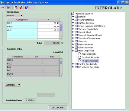
(1) Predictive Equation
In the [Conditions of Eq.] column and the [Property] field the conditions of restriction are shown.
(2) Compositional restrictions column (Condition of Eq.)
The conditions of restriction in glass composition are shown for the selected additivity equation.
(3) Field for composition input (Composition)
Input the names of components and their values.
Choose component names from the list opened by double-clicking in any cell of the Component column. Only usable components appear in the list. Input the content values by typing in values within the ranges shown in the compositional restriction column. Either mass% or mol% can be selected as the unit of composition, but it is recommended that the unit shown in the compositional restriction column be used.
(4) Property field
| * | Inputting conditions for calculation of the property (temperature and viscosity). It is necessary to input the temperature or viscosity for some additivity equations. When a white text box or pull-down menu appears, input or select the condition. The particular input condition depends on the additivity equation used. See Sec.1 of Chapter 5. |
| * | The unit system for this field can be changed. The default system is the Common unit system. However, this can be changed by setting the User Environment preferences accessed through the main window. |
| * | Representation of predictive value Pressing the [Calculate] button gives the predictive value resulting from the calculation. |
[Explanation of function]
(1) [Calculate] button
Select an additivity equation in the list. The conditions of restriction for the selected equation are shown in the property field. Click the [Calculate] button after inputting the temperature or viscosity as necessary. The predictive value is calculated. When the sum content of the components of a glass composition does not total 100 %, an alert appears to inform the user that the sum may be converted proportionally to total 100%.
Moreover, calculation is occasionally impossible even if the glass composition satisfies the stipulated restriction. In such cases, a warning message appears. See the 'special condition' for each additivity equation as shown in Sec.1 of Chapter 5.
(2)
[Print] icon Clicking on the printer icon prints the window as it appears.
| BACK | NEXT |